One year ago, Felt became the home of Tippecanoe, an open-source tool for creating vector map tiles from geographic data. Tippecanoe is a core component of our mapping stack at Felt. Ensuring our users get the best visualization of their data at every zoom level, no matter what file they upload gives us a rich set of problems to work on regularly, and development benefits our users as well as it’s open source community of users.
Two vexing algorithmic problems that have come up in the last several months have been how to choose good label points for polygons and how to simplify contiguous polygons without creating occasional shard gaps between them. In How Tippecanoe makes Felt's polygons look good, part 1: choosing good label points, I talked about how we choose unambiguous and visually pleasing label points for polygons on Felt maps in Tippecanoe. In this followup post I will talk about how we make the polygons themselves look as good as possible, while still operating efficiently on large data sets.
Continuous polygons
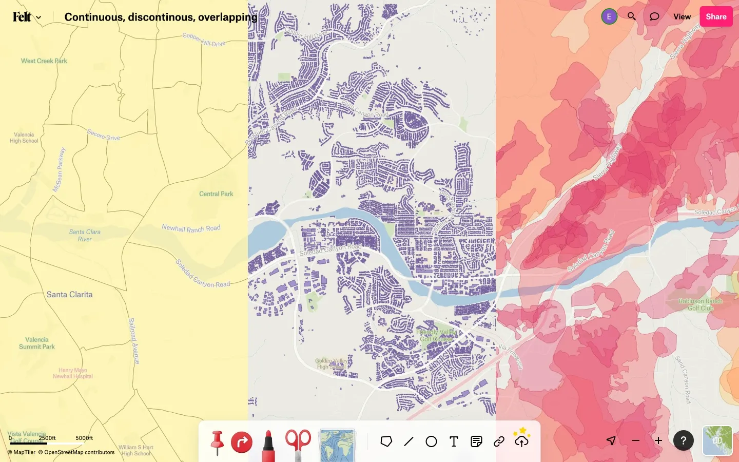
In particular, this post is about continuous polygons, like countries or states or census tracts or parcels, not discontinuous polygons, like typical building footprints, with gaps between the buildings, or overlapping polygons, like the areas affected by various natural disasters over the years, many of which overlap in their extents. (In a previous blog post I talked about Tippecanoe’s unusual “polygon dust” approach to representing discontinuous polygons at low zoom levels.) Here are examples of the three types: continuous census tracts, discontinuous buildings, and overlapping fire perimeters:
The specific visual expectation with continuous polygons is that the subject area of the map will be entirely filled with polygon features, with no gaps or overlaps between them, because this is the intent of the source data. The difficulty is that map users also expect generalization or simplification of the polygon shapes at low zoom levels, so that the map is not overwhelmed with irrelevant detail and does not look jarringly stairstepped or gridded. Each polygon geometry must be simplified, but to avoid creating overlaps or gaps between the polygons, each polygon must be simplified in exactly the same way as it its neighbors.
TopoJSON
At one level this is a thoroughly solved problem. In 2013, Mike Bostock released TopoJSON, a tool for finding the shared border segments between features in a GeoJSON file and simplifying them consistently, and described the algorithm that it uses. In 2016 I read his description and implemented it in Tippecanoe as the <p-inline>--detect-shared-borders<p-inline> option.
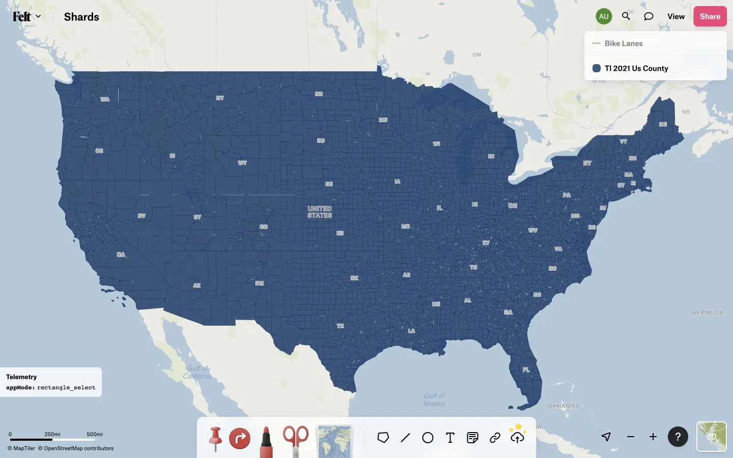
What’s the problem, then? The problem is that matching all the vertices of all of the features in a tile against each other, decomposing the feature geometries into arcs, simplifying each arc separately, and then reconstructing the features from the simplified arcs takes a lot of time and memory, enough so that I have always hesitated to recommend the use of the option, and enough so that it is impractical to use it on the large data sets that are often uploaded to Felt. As a result, until last month, continuous polygon maps on Felt would sometimes look like this, with small but visible gaps between the features:
Sorting as a way of life
How, then, can we get the benefits of topology-aware polygon simplification without the inefficiency of building in-memory data structures? There is a famous computer science paper in which Donald Knuth, asked to write a program to count the most frequently used words in a file, writes a beautiful, efficient program to track the words and their counts with a novel in-memory data structure, and Doug McIlroy responds with a one-line shell script that solves the same problem by transforming and sorting the source file and counting consecutive identical records in it.
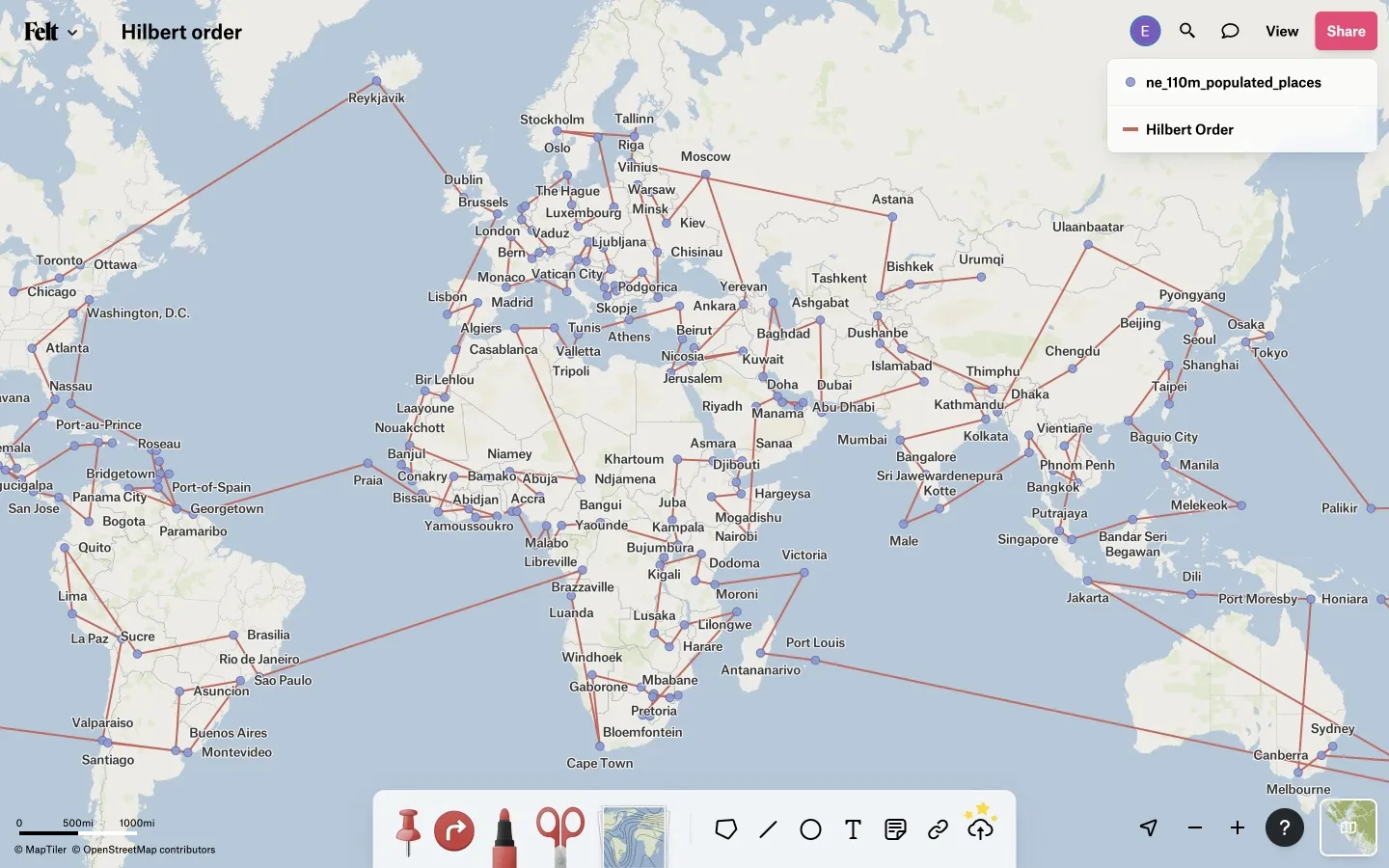
McIlroy’s way of looking at problems through the lens of sorting and scanning pervades Tippecanoe, which is entirely structured around the idea of sorting its input spatially into a file on disk (where “spatially” means handwavingly linearizing two-dimensional space into the Z-index or Hilbert value on the Mercator plane of some point within the feature), followed by sequentially reading that sorted stream and splitting it into smaller sorted streams, each of which is then again read sequentially and split into even smaller sorted streams, until the job of tiling is done.
There is no real spatial index, no real nearest-neighbor search, no real clustering, no real density calculation, only comparisons of consecutive elements of a sorted list being read from and rewritten into files on disk. This stream-oriented structure is what allows Tippecanoe to handle much larger inputs than can reasonably be stored in memory, a charmingly quaint notion in this decadent era of gigabytes of RAM in every pocket.
Topology by sorting
The recent changes to Tippecanoe similarly flatten topology into something that can be determined by a linear scan through a sorted file. In this case, instead of sorting features by a linearization of the location of a point within each feature, to associate it with the other data of for the feature, we sort vertices by a linearization of the location of each vertex within each feature, to associate the vertex with the two other vertices that it connects to.
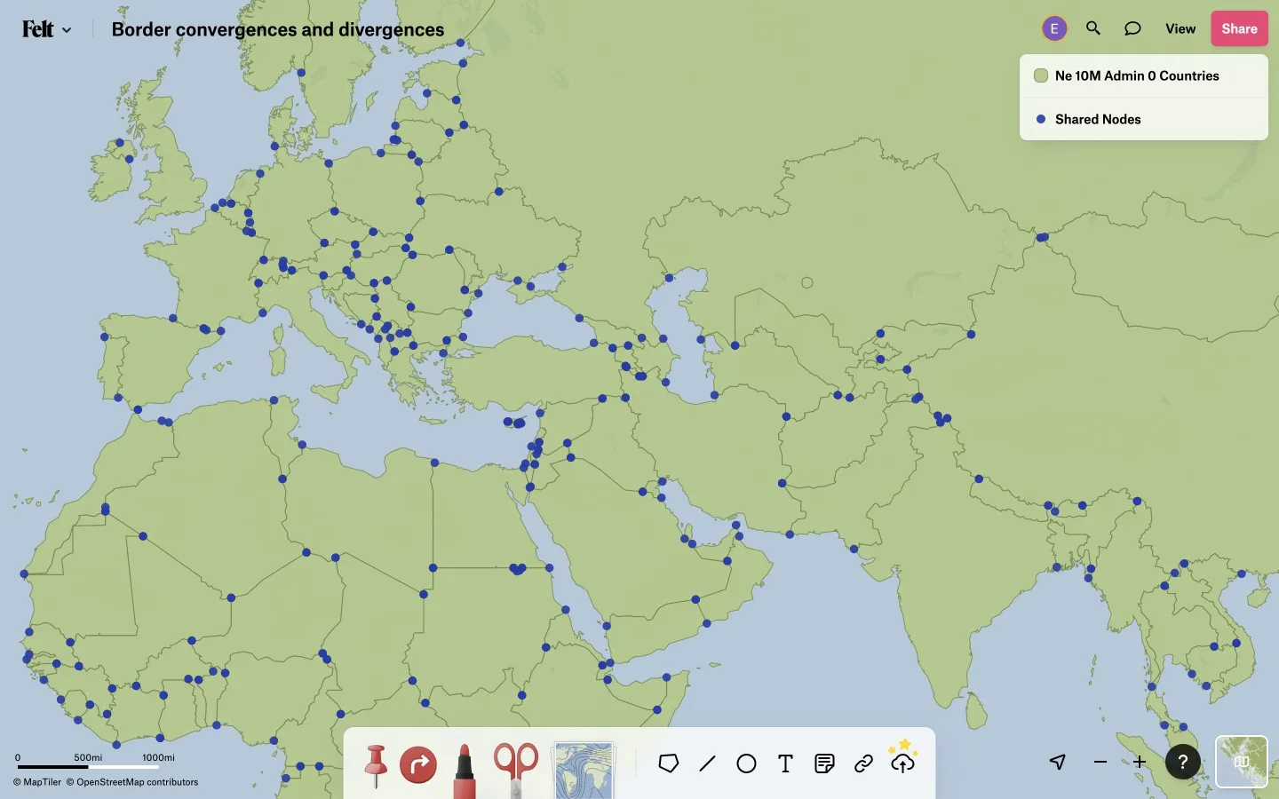
After sorting this list of vertices and their connections, we can scan through it linearly. If two consecutive records have the same central vertex but connect it to a different pair of adjacent vertices (taking into account that what is the previous vertex in one feature will be the next vertex in another, and vice versa), that central vertex is the point at which two polygon rings converge, diverge, or cross, and is therefore a point which must not be simplified away. These central vertices are written to a file of unsimplifiable nodes, also to be sorted and then searched later. This map shows some vertices at which national borders converge and diverge and which must not be simplified away:
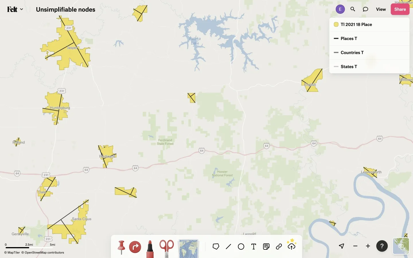
The other thing that is written to the file of unsimplifiable nodes is a set of three points chosen from each polygon ring, to make sure the ring is never simplified away to nothing (unless it is actually too small to display given the tile resolution), even if it doesn’t have enough significant vertices from its convergences and divergences with other features to keep it from collapsing into a line or a point from simplification. (Even in a map of generally continuous polygons, there are often isolated features, like islands, that do not connect with any other features.) These three points are intended to be the two ends of the major axis and a third point that is as far as possible from the line segment connecting the two axis points. Here are the three points that are chosen for each of some towns in Indiana:
Winding-neutral simplification
Once we have this sorted list of nodes that can never be simplified away, we can do simplification of polygon geometries without any further reference to the topology. We just need to do the old familiar Douglas-Peucker simplification on the outline of each polygon ring, with the additional caveat that any points in the ring that match a node in the list of unsimplifiable nodes must never be simplified away, in the same way that the starting and ending points of the geometry are never simplified away.
Unlike in TopoJSON, the polygons are not broken up into arcs, the arcs simplified, and the polygons then reconstructed from the arcs. In the Tippecanoe implementation, each polygon is simplified independently (and in parallel).
The tricky part is that when two polygons share a border, the vertices in that shared segment will be in the opposite order in one polygon than in the other, since the vertices in the outer ring of each polygon are always in clockwise order. The simplification algorithm therefore needs to take care to traverse the shared section in a consistent order, independent of the winding, and if two points are equally far from the segment connecting the endpoints of the segment, and are therefore equally likely to be chosen as the next point to retain into the final polygon, the tie must also be broken in a consistent way. Tippecanoe arbitrarily breaks these ties by comparing the Y coordinates of the points, or, if the two Y coordinates are equal, comparing the X coordinates.
The shards at right are big and bright
Perfection! Right? Well, no, actually, it is still possible for some overlaps and gaps to make it onto maps of continuous polygons, in spite of the good intentions of everything above.
The first way that this can happen, which should be fixed soon, is self-inflicted. Remember the “polygon dust” I mentioned above, which lets clusters of tiny polygons at low zoom levels be represented by larger combined placeholders? Well, sometimes those tiny polygons are supposed to be part of an area of continuous coverage, which will instead end up with holes in it where the tiny polygons were and an area of overlap around the larger placeholder.
This problem turns out to be solvable using the same information that is gathered above: if a polygon ring’s vertices contain four or more unsimplifiable nodes, it must share a border with another polygon, and therefore must not be allowed to be reduced to dust. The price it must pay in return for being saved from decay into dust is that if it gets simplified away to nothing because it is too small for the tile’s pixel grid, it gets no representation at all at this zoom level, unlike dust polygons which contribute to the size of the placeholder.
Preventing continuous polygons from decaying into dust makes an improvement in some cases, for instance between these two maps of Texas census blocks, in the first of which many gaps are visible in Dallas, Houston, and elsewhere:

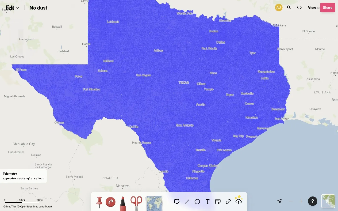
And yet even after this a few gaps remain in the second map. What is going on?
Seeking validation
The remaining source of geometric problems with continuous polygons is “polygon cleaning,” the final stage of processing before a polygon is added to a map tile. For correct display, MapLibre’s rendering of Felt maps depends upon valid, clean geometry for the features in each map tile. Among other things, this means that polygon geometries cannot have any self-intersections. All of the work above is to keep geometries consistent between features, and unfortunately does not make any guarantees about keeping geometries consistent within features, especially after they are scaled down from their original resolution to the resolution of each zoom level.
Tippecanoe relies on the Wagyu library to clean up polygon geometry after it is simplified and scaled, and Wagyu cannot avoid sometimes having to make slight changes to vertex locations to resolve conflicts within the geometry. Tippecanoe tries scaling the geometry back up before running Wagyu and then scaling it back down if all the vertices remained at integer coordinates, which sometimes produces better results than running it at tile resolution, but sometimes altering the locations of vertices can’t be avoided.
Here, for example, are some shard gaps between detailed precipitation contours that were introduced during polygon cleaning and that can be seen after rapidly zooming the map, before the better-looking higher-zoom-level tiles have had a chance to load:
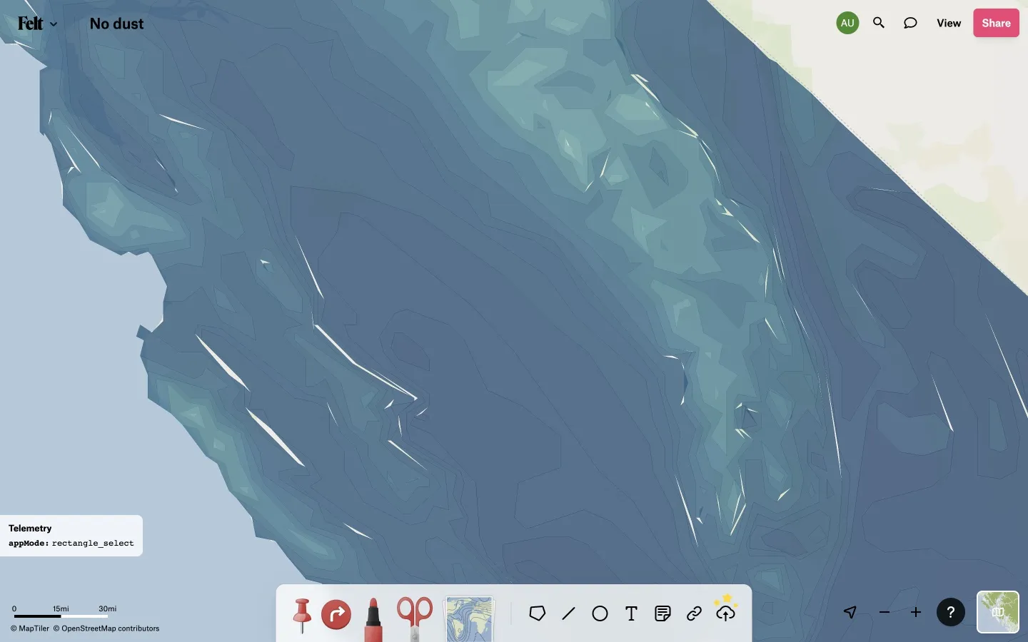
To really solve the problem, I think polygon cleaning will also need to be somewhat aware of topology, so that if a vertex has to be relocated or a new vertex has to be introduced to resolve an intersection conflict in one polygon, the corresponding change will also be made in the adjacent polygon. But that will have to wait until some other time.
Give it a try
Please upload your trickiest continuous polygons to Felt, or download Tippecanoe from GitHub or Homebrew and use the <p-inline>--no-simplification-of-shared-nodes<p-inline> option on them, and either enjoy your crisply simplified polygons or let me know if anything seems amiss.
Compare Felt using AI


.webp)