One year ago, Felt became the home of Tippecanoe, a geodata pre-processing tool that optimizes visual appearance across data densities and zoom levels to deliver fast web map tiles. Tippecanoe is a core component of our mapping stack at Felt. Ensuring our users get the best visualization of their data at every zoom level, no matter what file they upload, gives us a rich set of problems to work on regularly. Solutions benefit our users as well as Tippecanoe’s open source community of developers.

Two vexing algorithmic problems that have come up in the last several months have been how to quickly choose good label points for polygons and how to simplify contiguous polygons efficiently in large data sets without introducing shard gaps between them. This blog post will describe how we solved our label point problems; the simplification of contiguous polygons is covered in another post. Maptime and FOSS4G audience members were curious about how Tippecanoe generates label points, and I hope you will also find it interesting and perhaps applicable to other graphical applications. If you use Tippecanoe, a better understanding of what is going on inside it may help you make better maps.

Getting label points for polygons right

When users upload polygon data to Felt, each uploaded feature specifies the shape of the outline of each polygon, and often also specifies a text string, like a country or town name, to label the polygon with. But where within each polygon should the label be placed, to most clearly communicate which shape is being labeled, to cause the fewest conflicts with other labels, and to generally look the best? Making that decision is the job of a label placement algorithm.

Label anchors

The point on the map upon which each label is centered is sometimes called the “label anchor.” Felt used to generate label anchor locations for polygons by calling the representative_point function from the Shapely geometric analysis library, which in turn calls through to GEOS’s <p-inline>GEOSPointOnSurface<p-inline> function. Even though Shapely’s documentation refers to the representative point as “cheaply computed,” iterating through the features in Python to generate the label points was a significant enough performance bottleneck that we had to limit the number of labeled features per upload in order to be confident that uploads could finish processing in a reasonable amount of time.

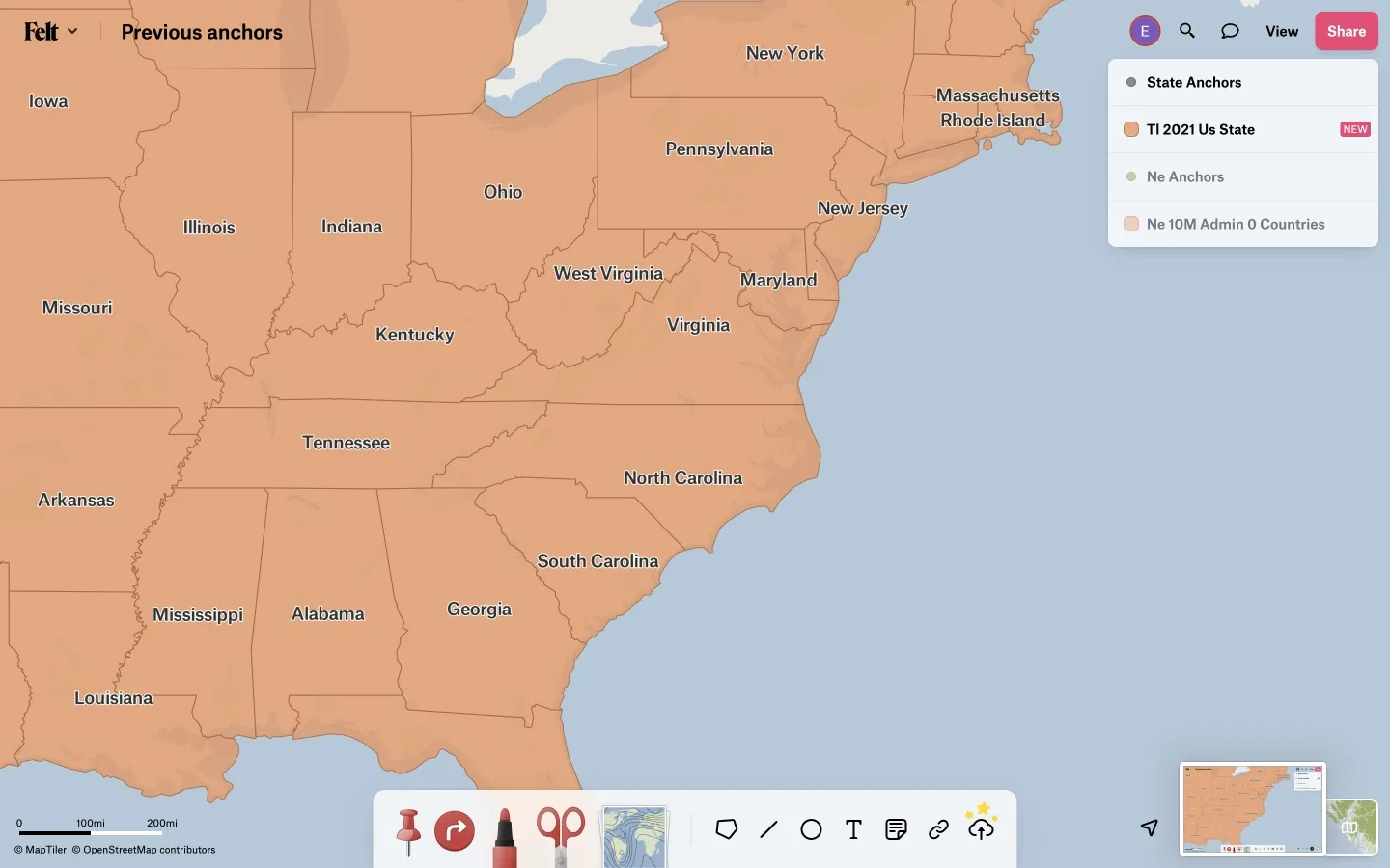
In addition, the points that were generated were sometimes confusing or aesthetically unsatisfying. The GEOS algorithm prefers to place a label close to the vertical center of a polygon ring, which is appropriate for many polygons, but sometimes results in some visual confusion, like these labels for Massachusetts and Louisiana that are right on the borders with Rhode Island and Mississippi.

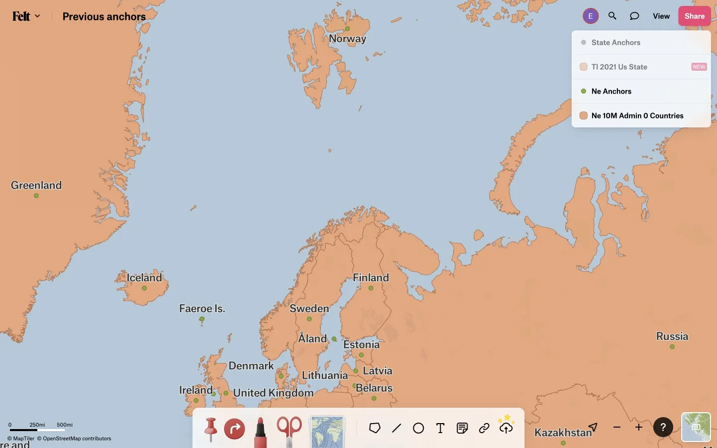
GEOS also sometimes also chooses a label point that is not in the largest ring of a MultiPolygon, resulting in surprising placements like this label for Norway, on Svalbard rather than on the mainland.

The function only yields a single label point per feature, which is appropriate for low zoom levels, but we also wanted some large features to have multiple labels when viewed at a higher zoom level, to reduce the distance that users would have to scroll to find the label. This desire for zoom level sensitivity made it seem appropriate to add label point generation to Tippecanoe, even if the speed of label generation could have been addressed through other existing tools.

Polylabel

My first thought for how to improve our label anchor generation was to try Polylabel, which is meant to generate optimal label points, located as far as possible from any border. Unfortunately, for the complex features that we accept as uploads, it can sometimes be quite slow. It also makes some surprising aesthetic choices, putting many of these state labels closer to one of the corresponding state’s borders than I would have expected.

Center of mass

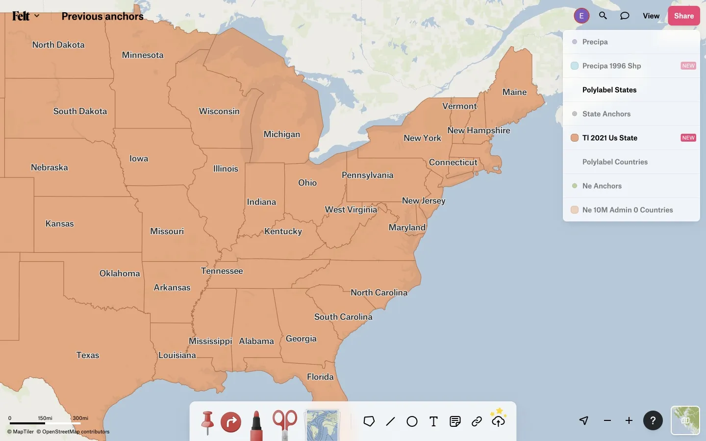
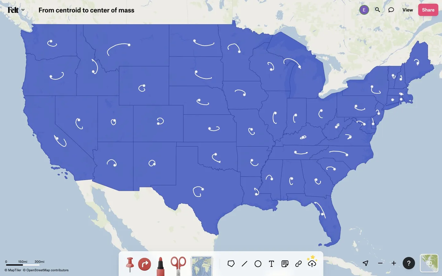
The best compromise between speed and aesthetically pleasing label placement frequently comes from Turf’s center-of-mass algorithm. It first calculates the centroid of the ring, and then walks around the edges, weighting the center of each edge by the area of the triangle connecting that edge to the centroid, following the formula given in Wikipedia. The point generated by applying this calculation to the polygon ring with the largest area is Tippecanoe’s top choice for the where to place the feature’s label. The map below shows the series of vectors whose sum leads from each contiguous US state’s centroid (the end of the tail) to its center of mass (the white dot), which is frequently a much more appealing location for a label than the centroid is.

Label point acceptance criteria

Unfortunately, sometimes the center of mass is still not an ideal place for a label. In a concave polygon, it may be outside of the bounds of the polygon, or in a polygon with a hole, it may be in a hole. To check the appropriateness of the label point, Tippecanoe uses the classic pnpoly algorithm to check whether the point is at a location with a positive fill, and also checks the distance of the point to each vertex and edge of the polygon. If it is in a hole or is closer to an edge or vertex than 1/5 of the radius that a circle with the same area as the polygon would have, the label point is rejected.

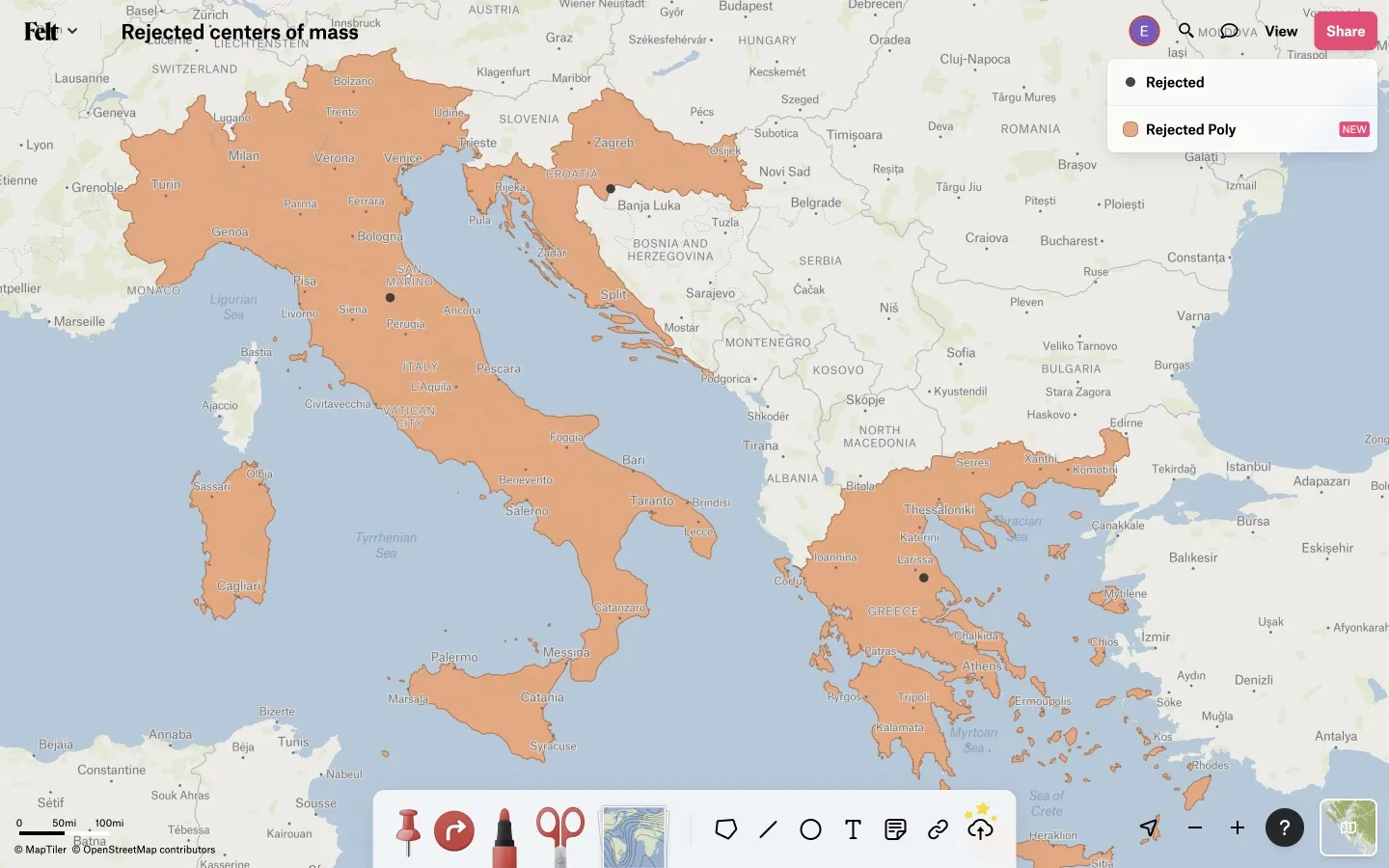
For example, the centers of mass of Italy, Croatia, and Greece are rejected as label points because they are too close to a border (in the case of Italy, too close to the enclave of San Marino), even though they are within the bounds of their respective countries.

Coordinate-sorted crossings

If the center of mass is not an acceptable point, Tippecanoe next tries a variation on GEOS’s vertical scan of the polygon. It sorts the vertices of the polygon in four ways: by Y coordinate, by X coordinate, and along two diagonals, with the expectation that in most cases successive sorted coordinates will bounce back and forth from one side of the polygon to the other, and then walks through pairs of coordinates in each of these orders. For each pair, it calculates the length and center of the segment. For example, it looks at these segments when trying to find an acceptable label point for Bermuda:

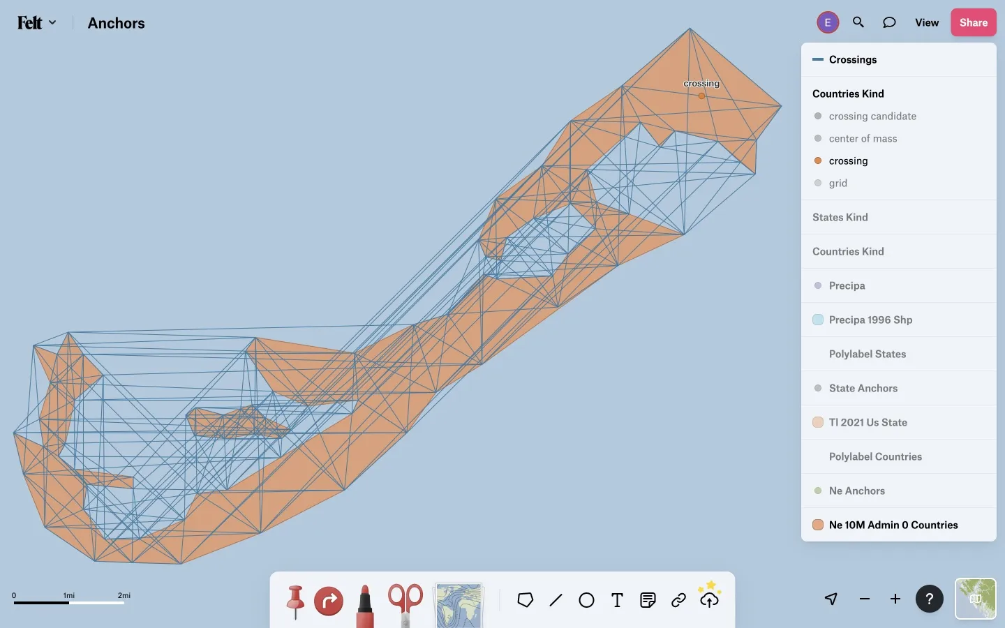
After collecting all of the crossings, it starts examining the midpoints, starting with the longest crossing, checking whether it meets the criteria above for being in the polygon interior and being acceptably far from a border. The first crossing that meets these criteria, if any, is accepted as the label point.

This search does not find as many good label point candidates as I had hoped it would. In retrospect it might have been better to triangulate the polygons as a source of diagonal crossings to consider as label points, and I will have to give that a try in a future version of Tippecanoe.

Grids

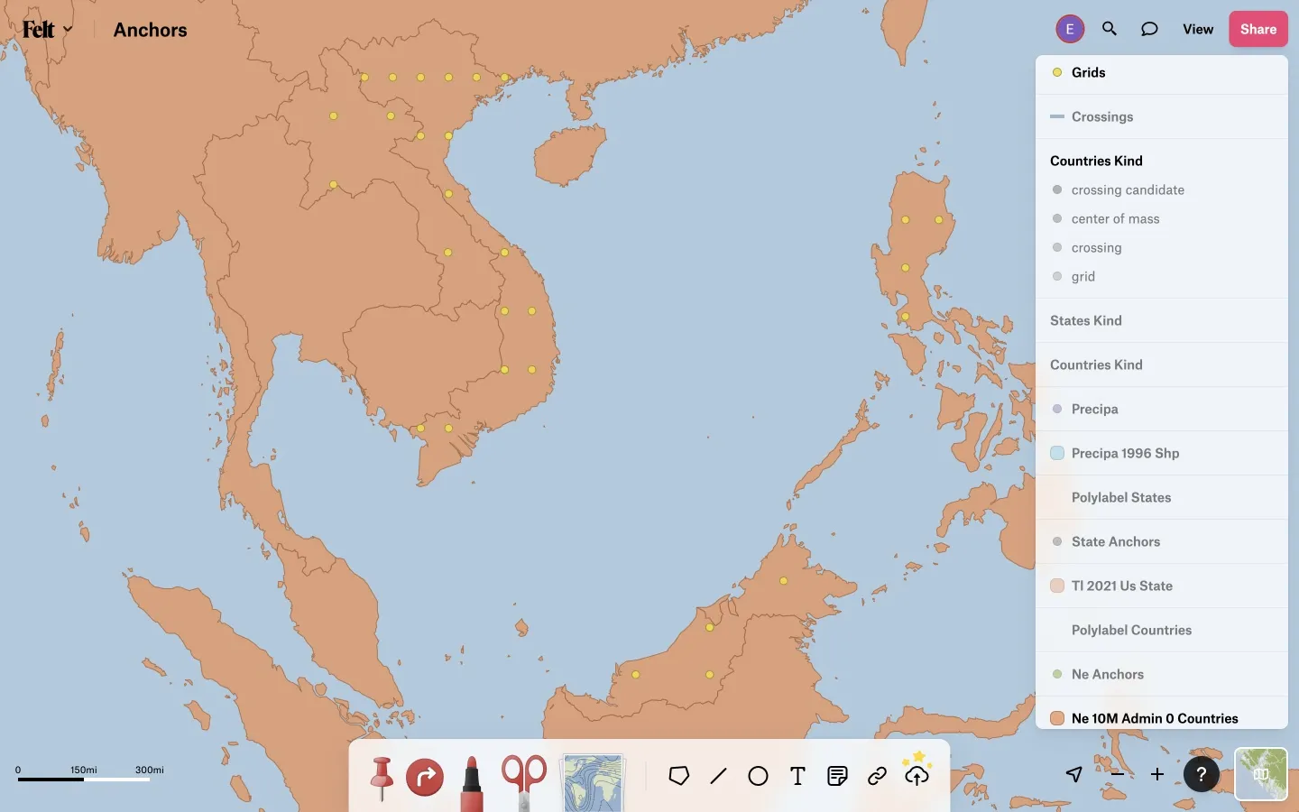
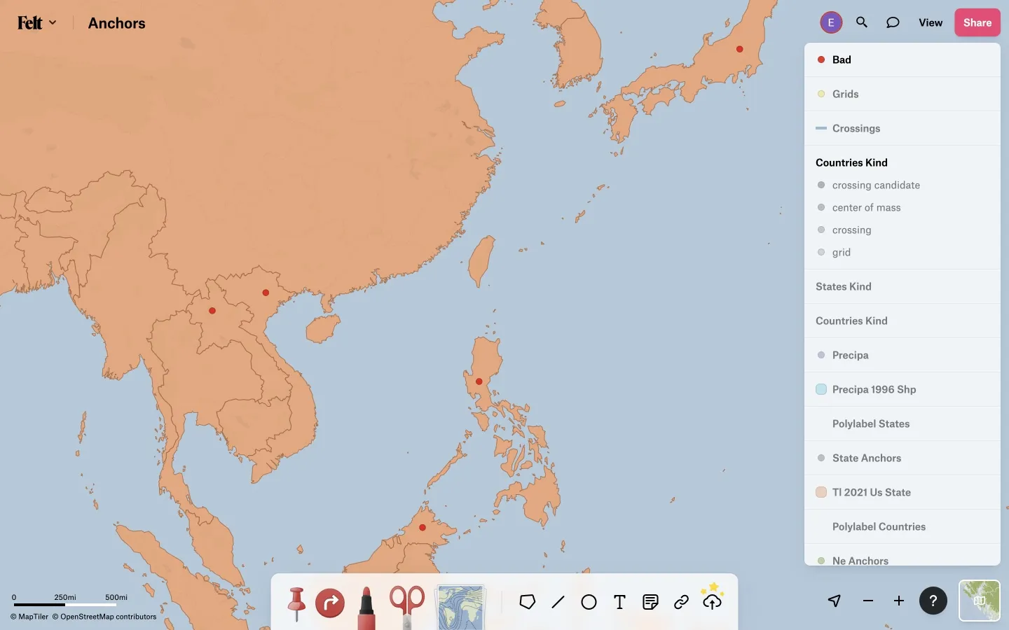
If no crossing produces an acceptable point, Tippecanoe then tries a series of gridded positions within the bounding box of the feature, starting with the center of the bounding box. If any of these meets the acceptance criteria, it is accepted as the label point. These are the grid points that are examined in the course of the search for acceptable label points for Vietnam, Laos, Malaysia, and the Philippines:

When nothing is satisfactory

If none of the above has produced an acceptable label point, Tippecanoe also tries the centroid of the vertices. If it meets the acceptance criteria, it is accepted as the label point; otherwise, whatever other point that has been tried that is in the feature interior and is the furthest from any edge or vertex is chosen as the best available. The points shown below were all too close to a border to have met the acceptance criteria, but were nevertheless better than any other points that were considered, so they were selected as the final label points:

Duplicate labels

As mentioned above, we wanted to make duplicate labels available in higher zoom levels so that users could orient themselves more easily. These are not subjected to the same high standard as the central label point; if an auxiliary label point candidate is outside the bounds of the polygon or is too close to a border, it is just dropped from consideration rather than prompting a search for another nearby point that would work.

We had originally decided to make the auxiliary labels spiral outward from the central label, but this proved to slow down tiling by creating too many extra label tiles at high zoom levels. Now instead we place the auxiliary labels in a simpler checkerboard pattern. For example, see the repeated “0”, “1000”, “2000”, and “3000” labels in this bathymetry map, with the single MultiPolygon feature for each ocean depth contour labeled multiple times.

Try it yourself

Please give the algorithms described above a try on your own polygon data, either by uploading it to a Felt map and turning on labels, or by installing Tippecanoe from Homebrew or Github and using the – convert-polygons-to-label-points option. If something doesn’t look as good as it ought to, please let me know so I can keep making our maps better.

The highest zoom levels, where these extra labels are generally most useful, are the same zoom levels at which it is extremely visible if the borders of adjacent polygons do not quite match up the way they should on the map. Rendering adjacent polygons identically, while still allowing geometries to be simplified to avoid a “stairstep” appearance, without using excessive time or memory, is another of the algorithmic challenges we have faced recently, and will be discussed in another upcoming blog post.